PostgreSQL is an open-source object-relational database that has been under development since 1986. It is characterized by ACID compliance, high extensibility, and strong SQL support. Companies value PostgreSQL for its reliability, performance, and cost-free nature. This guide answers the most important questions about the installation, configuration, and use of PostgreSQL in a corporate environment.
What is PostgreSQL and why do so many companies use it?

PostgreSQL is an object-relational database management system that is available as free open-source software. The database originated from the POSTGRES project at the University of California and has been continuously developed since 1986. PostgreSQL supports both relational and non-relational data structures and is considered one of the most advanced open-source databases worldwide.
The main features of PostgreSQL include ACID compliance for transaction security, Multi-Version Concurrency Control (MVCC) for concurrent access, and comprehensive SQL support. The database software also offers advanced data types such as JSON, XML, and arrays, as well as the ability to define custom functions and data types.
Companies of various sizes rely on PostgreSQL because it offers a stable and scalable solution for complex applications. The active developer community ensures regular updates and security patches. In addition, the free license allows for use without license costs, which is particularly attractive for growing companies.
How does PostgreSQL differ from other databases like MySQL?
PostgreSQL and MySQL differ in several important areas, with both having their specific strengths. PostgreSQL offers advanced data types such as JSON, JSONB, arrays, and geometric types, while MySQL focuses on basic SQL data types. PostgreSQL often shows better performance with complex queries and joins, while MySQL is often faster with simple read operations.
Licensing also differs: PostgreSQL is under the PostgreSQL license, which is very permissive, similar to the BSD license. MySQL uses dual licensing with GPL for open-source projects and commercial licenses for proprietary software. This can be relevant when deciding on commercial applications.
- PostgreSQL is particularly suitable for applications with complex data structures, analytical workloads, and when strict ACID compliance is required. For example, PostgreSQL natively supports geo-data and operations on geometric structures with the PostGIS extension.
- MySQL is often chosen for web applications, content management systems, and situations where simple configuration and high read performance are paramount.
Both databases have strong communities and professional support available.
What advantages does PostgreSQL offer for companies?
PostgreSQL offers companies significant cost advantages through the open-source license, as there are no license fees. This also enables small and medium-sized enterprises to build a professional database infrastructure. The saved license costs can be invested in hardware, development, or professional support.
PostgreSQL’s security standards meet enterprise requirements with features such as Row-Level-Security, SSL encryption, and comprehensive authentication options. The database supports various compliance standards and offers detailed audit functions for regulated industries.
PostgreSQL scales both vertically and horizontally and grows with the demands of your company. Independence from individual manufacturers prevents vendor lock-in and gives you the flexibility to obtain support and services from various providers. The large community and open development model ensure continuous innovation and long-term availability.
How to install and configure PostgreSQL correctly? Simple example:
The PostgreSQL installation is done in different ways depending on the operating system. Under Ubuntu/Debian, for example, use the command sudo apt-get install postgresql postgresql-contrib. For Windows, download the official installer from postgresql.org. macOS users can install PostgreSQL via Homebrew with brew install postgresql.
After the installation, you must start the PostgreSQL service and create a database user. Under Linux, this is done with sudo systemctl start postgresql and sudo -u postgres createuser --interactive. The basic configuration is done via the files postgresql.conf for general settings and pg_hba.conf for authentication.
This means that you are ready for a test on most Linux distributions. For more demanding applications, you should of course make further considerations, such as whether you want to rely on the packages and versions supplied with the respective distribution or whether you want to concentrate on the packages from PostgreSQL.org. A performant database server also requires considerations regarding the underlying file system and its optimization.
For productive use, you should also make important security settings:
- Change the default password of the postgres user, if one has been assigned
- Configure SSL encryption for network connections
- Restrict access via
pg_hba.confto necessary IP ranges - Enable logging for audit purposes
- Set up regular backups
How credativ® supports PostgreSQL projects
credativ® offers comprehensive PostgreSQL support for companies that need professional support for their database infrastructure. Our service includes 24/7 support from experienced PostgreSQL specialists who are immediately available for critical problems. You get direct access to our German support team without detours via international call centers. We are happy to help you and support you in the selection of open-source tools.
Our PostgreSQL services in detail:
- Migration from other database systems to PostgreSQL
- Installation consulting and audit of an existing installation
- Performance optimization and tuning of existing installations
- High availability setups with replication and clustering
- Backup and recovery strategies for maximum data security
- Monitoring and proactive maintenance of your PostgreSQL environment
- Long Term Support, which gives you time to complete the upgrades.
As PostgreSQL experts with over 20 years of experience, we help you to exploit the full potential of your database. Contact us for a non-binding consultation on your PostgreSQL project and find out how we can optimize your database infrastructure.
Postgres, PostgreSQL and the Slonik logo are trademarks or registered trademarks of the PostgreSQL Community Association of Canada and are used with their permission.
Foreman is clearly rooted in an IPv4 world. You can see it everywhere. Like it does not want to give you a host without IPv4, but without IPv6 is fine. But it does not have to be this way, so let’s go together on a journey to bring Foreman and the things around it into the present.
(more…)
credativ GmbH, a specialized service provider for open source solutions, is solidifying its position as a strategic partner for security-critical IT infrastructures. Since December 15, the company has been officially certified according to the international standards ISO/IEC 27001:2022 (Information Security) and ISO 9001:2015 (Quality Management).
Expertise from corporate structures – Agility as an independent company
This success is particularly remarkable, as credativ GmbH has only been operating independently on the market in its current form since March 1, 2025. The speed of certification within just nine months after the spin-off from NetApp Deutschland GmbH is no coincidence: the time within the corporate structures of NetApp was used specifically to build up in-depth know-how in highly regulated processes and global security standards.
A strong signal for public authorities and major clients
The certification covers all services provided by credativ GmbH. In doing so, the company creates a seamless basis of trust, which is essential, in particular, for cooperation with
Statements on the certification
David Brauner, Managing Director of credativ GmbH, emphasizes the strategic importance:
“Since our restart into independence on March 1, we have had a clear goal: to seamlessly transfer the high standards that we know from our time in the corporate environment into our new structure. The certification is a promise to our customers in the public sector and in the enterprise sector that we not only understand the high requirements for compliance and security, but also master them at the highest level.”
Alexander Wirt, CTO of credativ GmbH, adds:
“Quality and security are just as deeply rooted in us as the connection to open source. We have used the valuable experience from our time at NetApp to put our internal processes on a certifiable footing from day one. For our customers, this means that they receive the usual open source excellence, combined with the security of a partner working according to the most modern ISO standards.”
The advantages at a glance:
- Corporate-proven knowledge: Transfer of the highest compliance standards into an agile service environment.
- Highest data security: Protection of sensitive information according to the latest standard ISO/IEC 27001:2022.
- Verified process quality: Consistent management according to ISO 9001:2015 across all service areas.
- Ideal partner for the public sector: Fulfillment of all regulatory requirements for public authorities and critical infrastructures.
About credativ GmbH
credativ GmbH is an independent consulting and service company focusing on open source software. Following the spin-off from NetApp in spring 2025, credativ combines decades of community expertise with professional enterprise standards to make IT infrastructures secure, sovereign and future-proof, without losing the connection to its history of around 25 years of work in and with the open source community.

credativ is once again a Silver Member of the Linux Foundation. For us, this is not a symbolic gesture but a deliberate decision. For more than two decades, we have been working at the heart of open-source infrastructure – as a support center, as contributors, and as operators of critical services. Now that credativ is operating independently again, rejoining the Linux Foundation was one of our first strategic steps.
Why the Linux Foundation Matters to Us
The Linux Foundation is far more than the organizational home of the Linux kernel. It brings together essential building blocks of modern IT: cloud-native technologies such as Kubernetes, container ecosystems, security frameworks, and networking stacks. Many of these projects have become critical digital infrastructure.
Without neutral governance, transparent processes, and sustainable funding, these technologies would be markedly more vulnerable.
Digital Sovereignty and Resilience
Digital resilience is not accidental. It arises from stable structures, open development, and continuous maintenance. By supporting the Linux Foundation, we help ensure that essential software can be maintained reliably, updated securely, and developed independently.
Digital sovereignty means retaining control over one’s own data and infrastructure. Open Source is the prerequisite for that. The Linux Foundation provides the neutral space where technological progress can occur without dependence on individual vendors.
Our Contribution to the Ecosystem
Open Source only works when you give something back. Our teams contribute daily – packaging, debugging, upstream fixes, reviews, and operating systems that run in production environments around the globe.
Engagement in the Debian and PostgreSQL Communities
We have been active in the Debian community for many years: providing package maintenance, running essential infrastructure, and contributing to the project long-term. More information on our Debian involvement:
credativ & Debian
We also contribute significantly to the PostgreSQL ecosystem through consulting, support, technical development, and tooling. In addition, we support the community by sponsoring major events such as PGConf.EU.
More about our PostgreSQL work:
credativ PostgreSQL Competence Center
Open-Source Virtualization: Proxmox & ProxLB
Virtualization is becoming increasingly central to modern IT operations. We actively support the Proxmox community and contribute to ProxLB, an open-source load balancer for Proxmox VE.
An overview of our virtualization services:
Proxmox Virtualization at credativ
We also host the OSS Virtualisation Gathering, a community meetup focused on open virtualization technologies:
Meetup: OSS Virtualisation Gathering
Active Presence as Speakers at Open-Source Conferences
Our involvement does not end with code. We participate as speakers across many open-source conferences – in the Debian, PostgreSQL, Kubernetes, and Proxmox ecosystems.
Current reports and event recaps can be found on our blog:
credativ Blog
Following our initial announcement of the Open Source Virtualization Gathering this December, we are pleased to present the full agenda for the evening at our premises in Mönchengladbach today. A compact and informative exchange about open source virtualization with Proxmox VE and Ceph awaits you.
The meeting on 11 December 2025 will take place at the premises of credativ GmbH in Mönchengladbach:
credativ®
41179 Mönchengladbach, Germany

Agenda
Here is the planned schedule for the evening:
| Time | Item |
| 17:00 – 17:15 | Opening |
| 17:15 – 17:30 | Lecture: Ronald Otto, Managing Director of Tuxis B.V. on the topic of “Enterprise-Ready? How users deploy Proxmox VE and Ceph” (Lecture in English) |
| 17:30 – 17:45 | Time for questions and discussion |
| 17:45 – 18:00 | Coffee break and informal exchange |
| 18:00 – 18:30 | Lecture: Florian Paul Azim Hoberg (credativ) with “Proxmox VE as a virtualization engine for BoxyBSD” |
| 18:30 – 18:45 | Time for questions and discussion |
| 19:00 – 19:30 | Open section for questions and lightning talks |
| 19:30 – 19:45 | Closing (Official end) |
Actively shape the evening! The open section offers the ideal opportunity to contribute your own questions or short lightning talks (max. 5 minutes).
Following the official program, we cordially invite all participants to continue the exchange from 7:30 PM in the La Cottoneria on the ground floor (self-payers). Take the opportunity to network and benefit from the experiences of other participants.
Registration continues primarily via Meetup.com. For those who do not wish to register via Meetup.com, we alternatively offer the option of registering directly by email to info@credativ.de. Simply send us a short message to secure your place.
We look forward to welcoming you to Mönchengladbach!
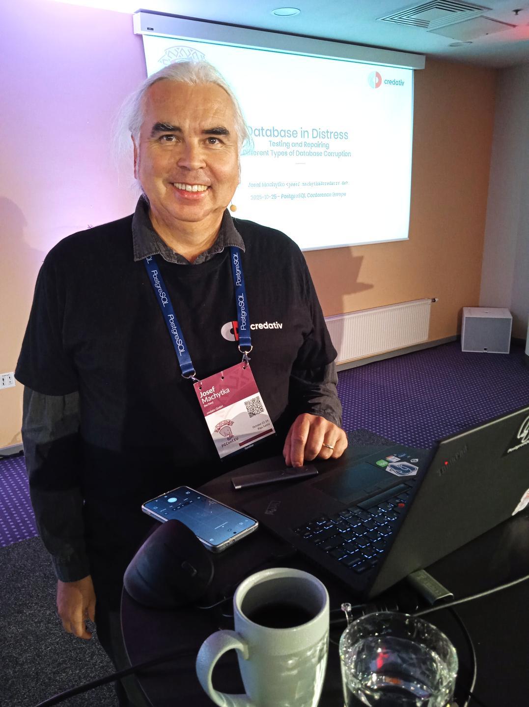
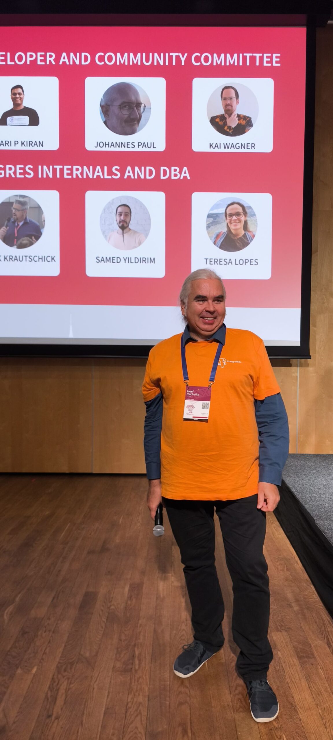
The European PostgreSQL Conference (PGConf.EU) is one of the largest PostgreSQL events worldwide. In this year it was held 21–24 October in Riga, Latvia. Our company, credativ GmbH, was a bronze sponsor of the conference, and I had the privilege to represent credativ with my talk “Database in Distress: Testing and Repairing Different Types of Database Corruption.” In addition, I volunteered as a session host on Thursday and Friday. The conference itself covered a wide range of PostgreSQL topics – from cloud-native deployments to AI integration, from large-scale migrations to resiliency. Below are highlights from sessions I attended, organised by day.
My talk about database corruption
I presenting my talk on Friday afternoon. In it I dove into real-world cases of PostgreSQL database corruption I encountered over the past two years. To investigate these issues, I built a Python tool that deliberately corrupts database pages and then examined the results using PostgreSQL’s pageinspect extension. During the talk I demonstrated various corruption scenarios and the errors they produce, explaining how to diagnose each case. A key point was that PostgreSQL 18 now enables data checksums by default at initdb. Checksums allow damaged pages to be detected and safely “zeroed out” (skipping corrupted data) during recovery. Without checksums, only pages with clearly corrupted headers can be automatically removed using the zero_damaged_pages = on setting. Other types of corruption require careful manual salvage. I concluded by suggesting improvements (in code or settings) to make recovery easier on clusters without checksums.
Tuesday: Kubernetes and AI Summits
Tuesday began with two half-day Summits. The PostgreSQL on Kubernetes Summit explored running Postgres in cloud-native environments. Speakers compared Kubernetes operators (CloudNativePG, Crunchy, Zalando, etc.), backup/recovery in Kubernetes, scaling strategies, monitoring, and zero-downtime upgrades. They discussed operator architectures and multi-tenant DBaaS use cases. Attendees gained practical insight into trade-offs of different operators and how to run Kubernetes-based Postgres for high availability.
In the PostgreSQL & AI Summit, experts examined Postgres’s role in AI applications. Topics included vector search (e.g. pgvector), hybrid search, using Postgres as context storage for AI agents, conversational query interfaces, and even tuning Postgres with machine learning. Presenters shared best practices and integration strategies for building AI-driven solutions with Postgres. In short, the summit explored how PostgreSQL can serve AI workloads (and vice versa) and what new features or extensions are emerging for AI use cases.
Wednesday: Migrations, Modelling, and Performance
Joaquim Oliveira (European Space Agency) discussed moving astronomy datasets (from ESA’s Gaia and Euclid missions) off Greenplum. The team considered both scaling out with Citus and moving to EDB’s new Greenplum-based cloud warehouse. He covered the practical pros and cons of each path and the operational changes required to re-architect such exascale workloads. The key lesson was planning architecture, tooling, and admin shifts needed before undertaking a petabyte-scale migration.
Boriss Mejias (EDB) emphasised that data modelling is fundamental to software projects. Using a chess-tournament application as an example, he showed how to let PostgreSQL enforce data integrity. By carefully choosing data types and constraints, developers can embed much of the business logic directly in the schema. The talk demonstrated “letting PostgreSQL guarantee data integrity” and building application logic at the database layer.
Roberto Mello (Snowflake) reviewed the many optimizer and execution improvements in Postgres 18. For example, the planner now automatically eliminates unnecessary self-joins, converts IN (VALUES…) clauses into more efficient forms, and transforms OR clauses into arrays for faster index scans. It also speeds up set operations (INTERSECT, EXCEPT), window aggregates, and optimises SELECT DISTINCT and GROUP BY by reordering keys and ignoring redundant columns. Roberto compared query benchmarks across Postgres 16, 17, and 18 to highlight these gains.
Nelson Calero (Pythian) shared a “practical guide” for migrating 100+ PostgreSQL databases (from gigabytes to multi-terabytes) to the cloud. His team moved hundreds of on-prem VM databases to Google Cloud SQL. He discussed planning, downtime minimisation, instance sizing, tools, and post-migration tuning. In particular, he noted challenges like handling old version upgrades, inheritance schemas, PostGIS data, and service-account changes. Calero’s advice included choosing the right cloud instance types, optimising bulk data loads, and validating performance after migration.
Jan Wieremjewicz (Percona) recounted implementing Transparent Data Encryption (TDE) for Postgres via the pg_tde extension. He took the audience through the entire journey – from the initial idea, through patch proposals, to community feedback and design trade-offs. He explained why existing PostgreSQL hooks weren’t enough, what friction was encountered, and how customer feedback shaped the final design. This talk served as a “diary” of what it takes to deliver a core encryption feature through the PostgreSQL development process.
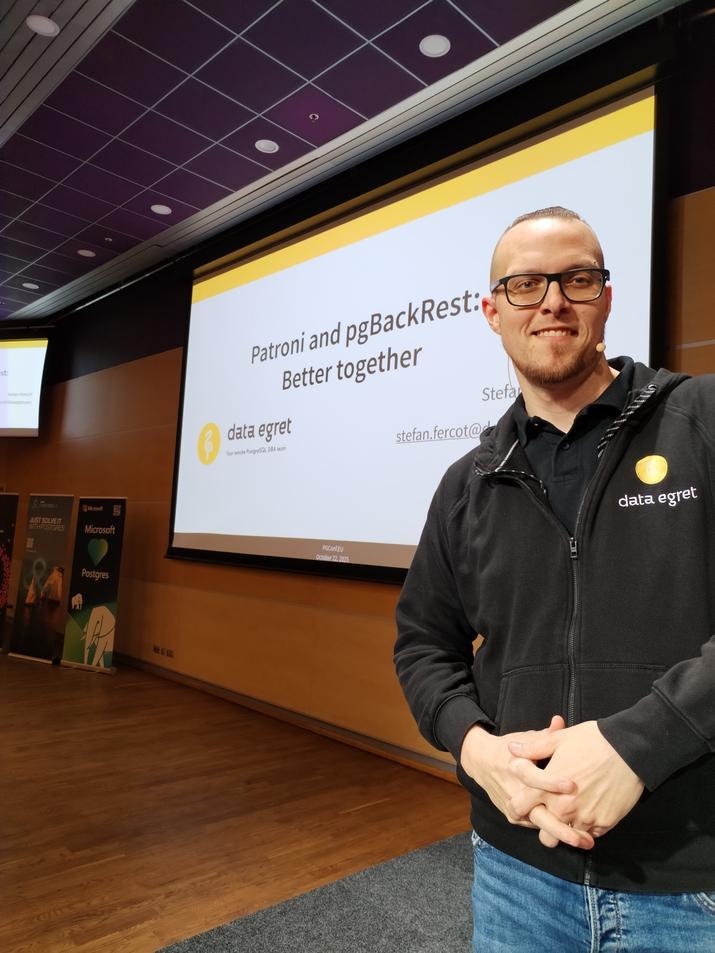
Stefan Fercot (Data Egret) demonstrated how to use Patroni (for high availability) together with pgBackRest (for backups). He walked through YAML configuration examples showing how to integrate pgBackRest into a Patroni-managed cluster. Stefan showed how to rebuild standby replicas from pgBackRest backups and perform point-in-time recovery (PITR) under Patroni’s control. The talk highlighted real-world operational wisdom: combining these tools provides automated, repeatable disaster recovery for Postgres clusters.
Thursday: Cloud, EXPLAIN, and Resiliency
Maximilian Stefanac and Philipp Thun (SAP SE) explained how SAP uses PostgreSQL within Cloud Foundry (SAP’s open-source PaaS). They discussed optimisations and scale challenges of running Postgres for SAP’s Business Technology Platform. Over the years, SAP’s Cloud Foundry team has deployed Postgres on AWS, Azure, Google Cloud, and Alibaba Cloud. Each provider’s offerings differ, so unifying automation and monitoring across clouds is a major challenge. The talk highlighted how SAP contributes Postgres performance improvements back to the community and what it takes to operate large-scale, cloud-neutral Postgres clusters.
In “EXPLAIN: Make It Make Sense,” Aivars Kalvāns (Ebury) helped developers interpret query plans. He emphasized that after identifying a slow query, you must understand why the planner chose a given plan and whether it is optimal. Aivars walked through EXPLAIN output and shared rules of thumb for spotting inefficiencies – for example, detecting missing indexes or costly operators. He illustrated common query anti-patterns he has seen in practice and showed how to rewrite them in a more database-friendly way. The session gave practical tips for decoding EXPLAIN and tuning queries.
Chris Ellis (Nexteam) highlighted built-in Postgres capabilities that simplify application development. Drawing on real-world use cases – such as event scheduling, task queues, search, geolocation, and handling heterogeneous data – he showed how features like range types, full-text search, and JSONB can reduce application complexity. For each use case, Chris demonstrated which Postgres feature or data type could solve the problem. This “tips & tricks” tour reinforced that leveraging Postgres’s rich feature set often means writing less custom code.
Andreas Geppert (Zürcher Kantonalbank) described a cross-cloud replication setup for disaster resilience. Faced with a requirement that at most 15 minutes of data could be lost if any one cloud provider failed, they could not use physical replication (since their cloud providers don’t support it). Instead, they built a multi-cloud solution using logical replication. The talk covered how they keep logical replicas up-to-date even as schemas change (noting that logical replication doesn’t automatically copy DDL). In short, logical replication enabled resilient, low-RPO operation across providers despite schema evolution.
Derk van Veen (Adyen) tackled the deeper rationale behind table partitioning. He emphasised the importance of finding the right partition key – the “leading figure” in your data – and then aligning partitions across all related tables. When partitions share a common key and aligned boundaries, you unlock multiple benefits: decent performance, simplified maintenance, built-in support for PII compliance, easy data cleanup, and even transparent data tiering. Derk warned that poorly planned partitions can hurt performance terribly. In his case, switching to properly aligned partitions (and enabling enable_partitionwise_join/_aggregate) yielded a 70× speedup on 100+ TB financial tables. All strategies he presented have been battle-tested in Adyen’s multi-100 TB production database.
Friday: Other advanced Topics
Nicholas Meyer (Academia.edu) introduced thin cloning, a technique for giving developers real production data snapshots for debugging. Using tools like DBLab Engine or Amazon Aurora’s clone feature, thin cloning creates writable copies of live data inexpensively. This lets developers reproduce production issues exactly – including data-dependent bugs – by debugging against these clones of real data. Nicholas explained how Academia.edu uses thin clones to catch subtle bugs early by having dev and QA teams work with near-production data.
Dave Pitts (Adyen) explained why future Postgres applications may use both B-tree and LSM-tree (log-structured) indexes. He outlined the fundamental differences: B-trees excel at point lookups and balanced reads/writes, while LSM-trees optimise high write throughput and range scans. Dave discussed “gotchas” when switching workloads between index types. The talk clarified when each structure is advantageous, helping developers and DBAs choose the right index for their workload.

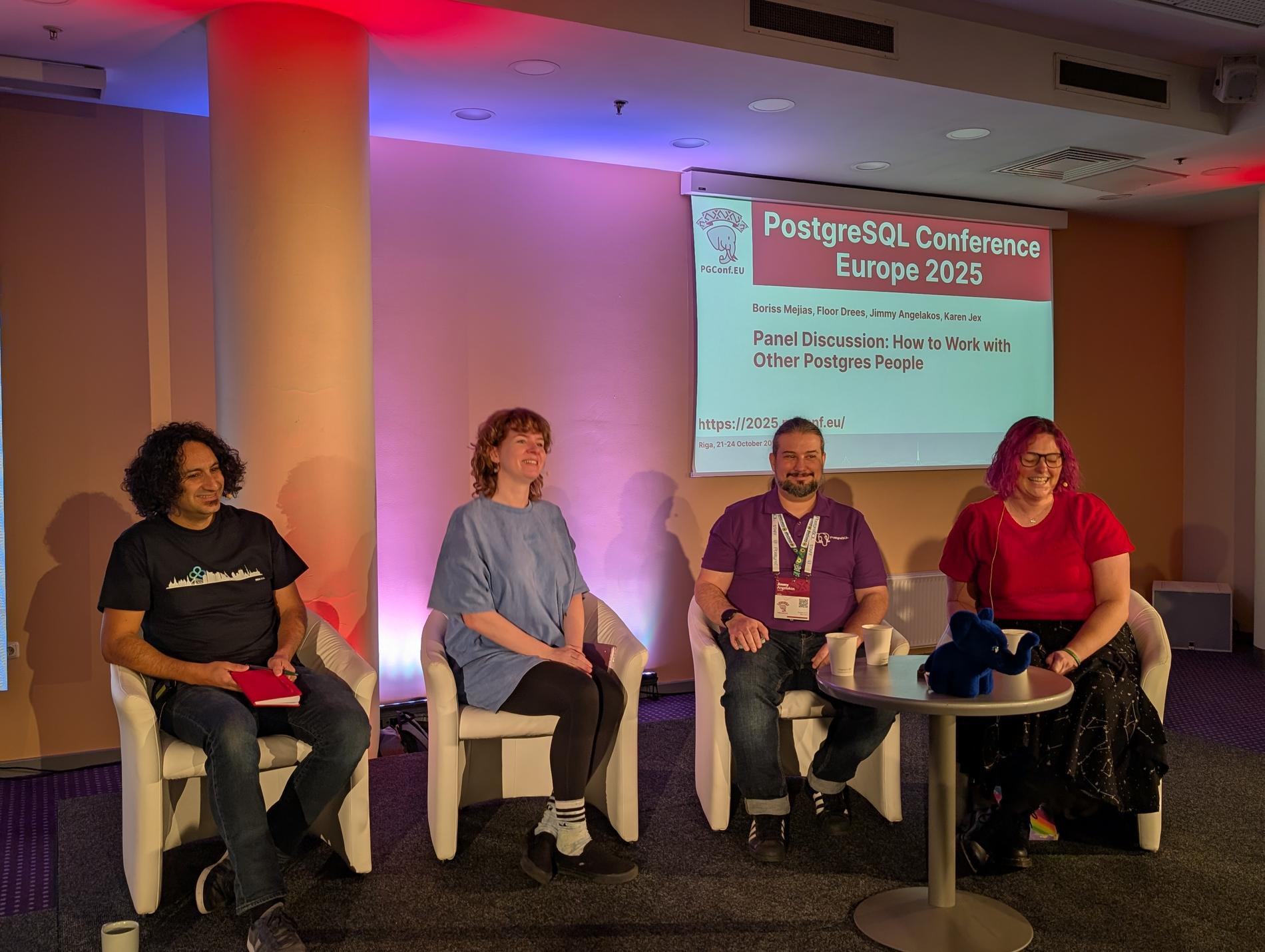
A panel led by Jimmy Angelakos addressed “How to Work with Other Postgres People”. The discussion focused on mental health, burnout, and neurodiversity in the PostgreSQL community. Panelists highlighted that unaddressed mental-health issues cause stress and turnover in open-source projects. They shared practical strategies for a more supportive culture: personal “README” guides to explain individual communication preferences, respectful and empathetic communication practices, and concrete conflict resolution techniques. The goal was to make the Postgres community more welcoming and resilient by understanding diverse needs and supporting contributors effectively.
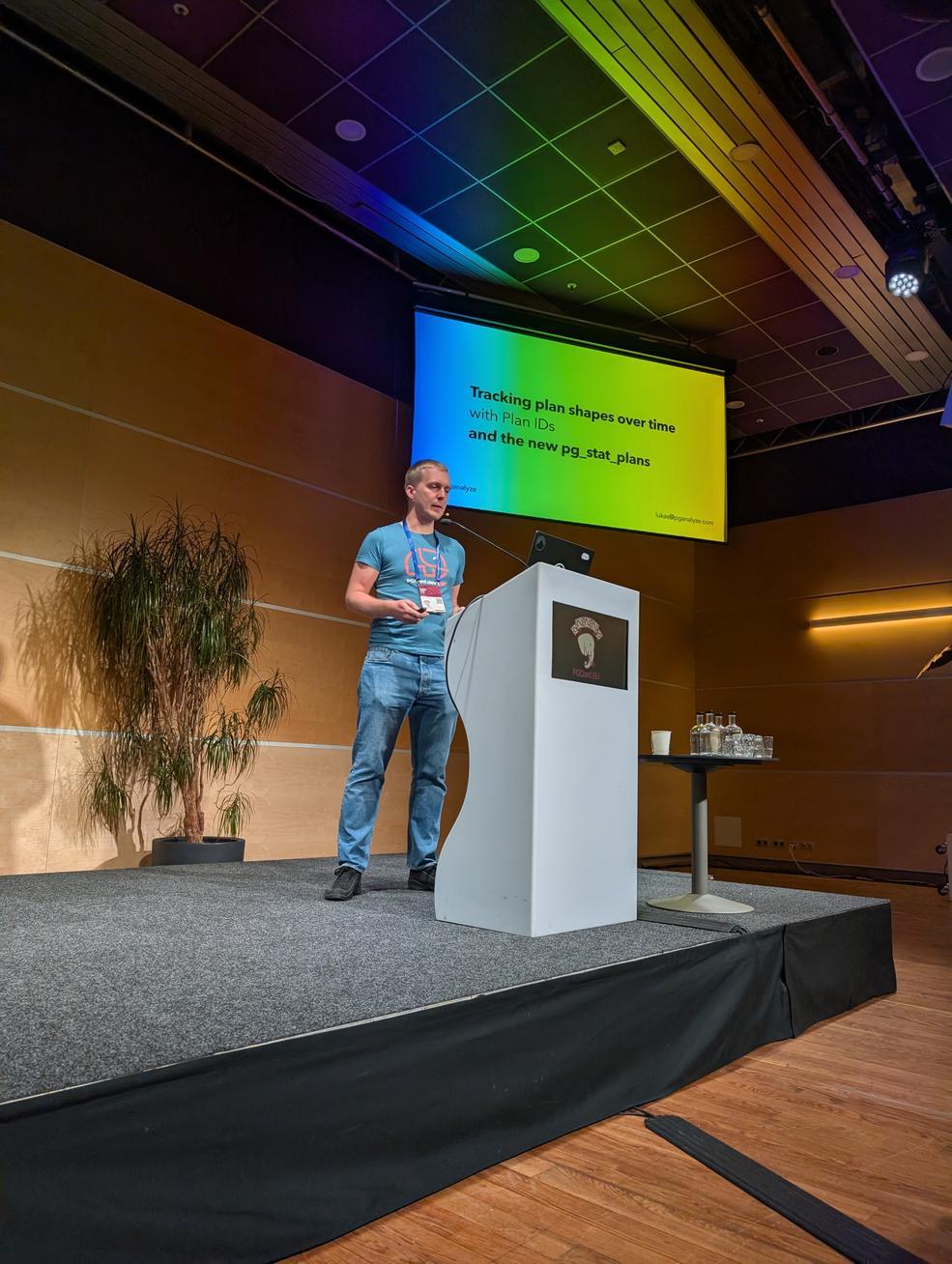
Lukas Fittl (pganalyze) presented new tools for tracking query plan changes over time. He showed how to assign stable Plan IDs (analogous to query IDs) so that DBAs can monitor which queries use which plan shapes. Lukas introduced the new pg_stat_plans extension (leveraging Postgres 18’s features) for low-overhead collection of plan statistics. He explained how this extension works and compared it to older tools (the original pg_stat_plans, pg_store_plans, etc.) and cloud provider implementations. This makes it easier to detect when a query’s execution plan changes in production, aiding performance troubleshooting.
Ahsan Hadi (pgEdge) described pgEdge Enterprise PostgreSQL, a 100% open-source distributed Postgres platform. pgEdge Enterprise Postgres provides built-in high availability (using Patroni and read replicas) and the ability to scale across global regions. Starting from a single-node Postgres, users can grow to a multi-region cluster with geo-distributed replicas for extreme availability and low latency. Ahsan demonstrated how pgEdge is designed for organizations that need to scale from single instances to large distributed deployments, all under the standard Postgres license.
Conclusion
PGConf.EU 2025 was an excellent event for sharing knowledge and learning from the global PostgreSQL community. I was proud to represent credativ and to help as a volunteer, and I’m grateful for the many insights gained. The sessions above represent just a selection of the rich content covered at the conference. Overall, PostgreSQL’s strong community and rapid innovation continue to make these conferences highly valuable. I look forward to applying what I learned in my work and to attending future PGConf.EU events.
This December, we are launching the very first Open Source Virtualization Meeting, also known as the Open Source Virtualization Gathering!
Join us for an evening of open exchange on virtualization with technologies such as KVM, Proxmox, and XCP-ng.
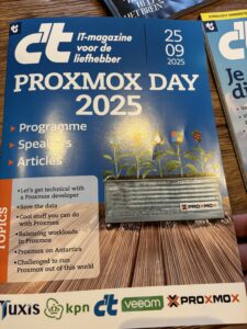
Review of the Dutch Proxmox Day 2025
On September 25, 2025, we attended the Dutch Proxmox Day 2025 in Ede (Netherlands) – and I must say: the event was a complete success. Organized by Tuxis B.V. at the Hotel Belmont in the Veluwe region, the day offered an excellent mix of expert presentations and valuable exchange.
Thanks to the Hosts
A heartfelt thank you to the Tuxis team: For the invitation as a speaker, for the trust placed in us, and for the perfect organization. Yes — this blog article is coming a bit late, but as they say: better late than never.
My Perspective as a Speaker
As a speaker, I had the pleasure of being part of an exciting program. At the same time, I was a participant: both at the same time – that’s what makes such days special. I would like to highlight a few presentations:
- Aaron Lauterer (Linux Software Developer at Proxmox Server Solutions) – “Let’s get technical with a Proxmox developer”: A look at upcoming features of Proxmox VE. The upcoming integration of OCI containers (aka Docker) is particularly exciting.
- Rob Turk (Senior Presales Systems Engineer at Veeam) – “Save the data”: Clearly shows that Proxmox has now arrived in the enterprise world.
- Mark Schouten (CTO at Tuxis) – “Cool stuff you can do with Proxmox”: Proxmox Backup Server in interaction with ZFS, how to make the whole thing more performant and what unexpected problems with SCSI and Western Digital have occurred, Mark Schouten told us about it
- Alexander Wirt – “Balancing workloads in Proxmox”: My own contribution with a focus on the project ProxLB of my esteemed colleague Florian Hoberg, which distributes virtual machines evenly across nodes, again shows the advantages and OSS and open interfaces. These make it easy to add missing functionality and thus compete with the industry giants.
- Robbe Van Herck (Support & Maintenance Engineer at International Polar Foundation) – “Proxmox on Antarctica”: Proxmox in extreme use – at the other end of the world and very far from everyday data center life. Robbe was able to show well that Proxmox also works in the most remote corners of the earth, the other challenges are more exciting here – such as hardware that is overwhelmed by the low temperatures.
- Han Wessels (Operations System Engineer at ESA) – “Challenged to run Proxmox out of this world”: Why Proxmox can also be operated on the ISS or in space – technology meets vision. Han vividly described the challenges that arise, such as the vibration during the launch of the carrier rocket or the radiation that significantly shortens the lifespan of storage.
I was able to take away many impulses – both technically and ideally. And I had good conversations that will certainly pay off further.
Networking & Exchange
The informal part was just as valuable as the program: during the breaks, at lunch or at the get-together in the afternoon, we made new contacts, gained interesting insights and met old acquaintances. It is precisely these moments that make a conference come alive.
Outlook
We are already looking forward to next year. When the Tuxis team calls again, we will be happy to be there again. Many thanks again to all those involved, all speakers and all participants – see you again. In between, this December there will be the first Open Source Virtualization Gathering at our company.
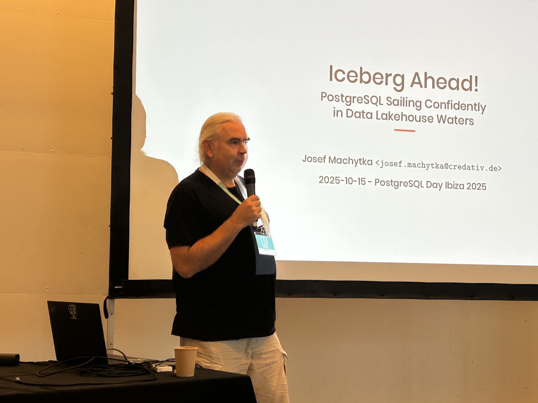
Postgres Ibiza 2025 took place on October 15–17, 2025, at the Palacio de Congresos de Ibiza on the beautiful island of Ibiza in the Mediterranean Sea. The conference is organized by the Spanish non‑profit Fundación PostgreSQL and aims to be a “refreshing, open and diverse Postgres conference” in a “truly unique environment.” And sure enough, the event is intentionally remarkable, organizers curate talks on cutting‑edge topics. The conference spans three days: the first two are devoted to scheduled talks, and the last day is an “unconference workshop day,” where participants propose and vote on topics to discuss.
I had the pleasure of representing our company credativ GmbH with talk, “Iceberg Ahead! PostgreSQL Sailing Confidently in Data Lakehouse Waters.” This was the fourth, heavily updated version of my already very successful talk on PostgreSQL and data lakehouses; earlier versions this year appeared at P2D2 2025 in Prague, PGConf.DE 2025 in Berlin, and Swiss PGDay 2025 in Rapperswil‑Jona. This latest version, developed specifically for Postgres Ibiza, dives deep into the Parquet data format, its use in Apache Iceberg tables, and how PostgreSQL can integrate with it using various extensions and tools.
But every single talk at this conference was interesting and high‑quality. I especially enjoyed these:
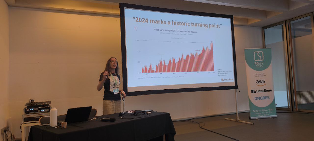
- Keynote from Catherine Bouxin (Data Bene) — “Reduce energy usage: contributing towards a greener future while directly improving cost and performance.” She highlighted how IT has become a huge consumer of energy, contributing to climate change—and why every optimization matters. It’s a topic not often discussed in the IT world and it drew a lot of attention from the audience.
- Robert Treat — “Vacuuming Large Tables: How Recent Postgres Changes Further Enable Mission Critical Workloads.” He presented a scary real‑life scenario—a vacuum failure turned into a steep learning opportunity—and explained how to avoid transaction wraparound disasters on extremely high‑load systems.
- Mauricio Zambrano — “PostgreSQL at the Square Kilometre Array Observatory.” The SKAO is a massive global radio‑telescope project, gathering extreme amounts of data every second. Managing this unbelievable data flow with PostgreSQL on Kubernetes is truly a cosmic challenge.
- Álvaro Hernández — “Postgres à la carte: dynamic container images with your choice of extensions.” He presented a new approach to dynamic container images that lets users add whatever PostgreSQL extensions they need without maintaining special custom images for every combination.
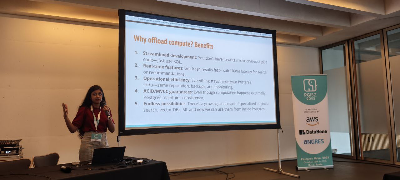
- Sweta Vooda — “Beyond Storage: Postgres as a Control Plane.” This session reimagined what we can do with Postgres beyond just storing data. She showed patterns and ideas for building extensions that let PostgreSQL orchestrate external compute engines, offloading heavy workloads to specialized systems.
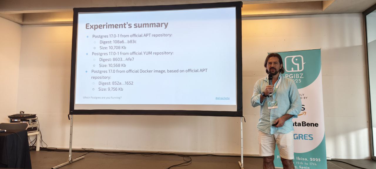
- On the second day, Álvaro Hernández delivered the keynote “Which Postgres are you running?” about why it’s crucial to know the exact build of PostgreSQL you run. He discussed reproducible builds and SBOMs (Software Bill of Materials), and introduced a new idea for a more reliable solution.
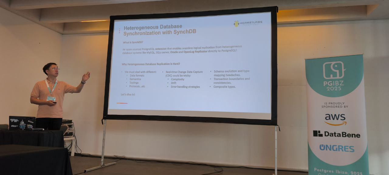
- Grant Zhou — “Universal Database Synchronization with Modern Multi‑Connector Architecture.” He introduced the SynchDB extension, which can perform CDC from multiple sources—MySQL, SQL Server, and Oracle—into PostgreSQL.
- Cédric Villemain — “Stats roll, baby, stats roll.” He explained the new PACS framework for advanced PostgreSQL observability.
- And last but not least, Michael Meskes — “From Code to Commerce: Open Source Business Models.” A long‑time open‑source entrepreneur and founder of credativ, he offered thoughtful insights into business models from dual‑licensing to open‑core to newer cloud/SaaS approaches, with pros and cons for each.
- Challenges and solutions for migration from Oracle to PostgreSQL, including performance optimizations and replacement of Oracle‑specific code
- Different database benchmarks and their use cases, pitfalls and relevance for different use cases
- Migration validation methods
- PostgreSQL extensions development – experiences and best practices
- PostgreSQL observability and monitoring tools
- Growing the next generation of PostgreSQL hackers and contributors
Postgres Ibiza was both technically enriching and personally enjoyable. It’s an inspiring place to recharge your enthusiasm for technology in a deeply inspiring environment while listening to and discussing engaging topics. The small, cozy setting allows for deep, meaningful conversations with everyone—and for making new friends. I’m already looking forward to next year’s edition of this amazing conference!
 On September 4, 2025, the third pgday Austria took place in the Apothecary Wing of Schönbrunn Palace in Vienna, following the previous events in 2021 and 2022.
153 participants had the opportunity to attend a total of 21 talks and visit 15 different sponsors, discussing all possible topics related to PostgreSQL and the community.
Also present this time was the Sheldrick Wildlife Trust, which is dedicated to rescuing elephants and rhinos. Attendees could learn about the project, make donations, and participate in a raffle.
The talks ranged from topics such as benchmarking and crash recovery to big data.
Our colleague was also represented with his talk “Postgres with many data: To MAXINT and beyond“.
As a special highlight, at the end of the day, before the networking event, and in addition to the almost obligatory lightning talks, there was a “Celebrity DB Deathmatch” where various community representatives came together for a very entertaining stage performance to find the best database in different disciplines. To everyone’s (admittedly not great) surprise, PostgreSQL was indeed able to excel in every category.
Additionally, our presence with our own booth gave us the opportunity to have many very interesting conversations and discussions with various community members, as well as sponsors and visitors in general.
For the first time, the new managing director of credativ GmbH was also on site after our re-independence and saw things for himself.
All in all, it was a (still) somewhat smaller, but nonetheless, as always, a very instructive and familiar event, and we are already looking forward to the next one and thank the organizers and the entire team on site and behind the scenes.
Dear Open Source Community, dear partners and customers,
We are pleased to announce that credativ GmbH is once again a member of the Open Source Business Alliance (OSBA) in Germany. This return is very important to us and continues a long-standing tradition, because even before the acquisition by NetApp,
The OSBA
OSBA aims to strengthen the use of Open Source Software (OSS) in businesses and public administration. We share this goal with deep conviction. Our renewed membership is intended not only to promote networking within the community but, above all, to support the important work of the OSBA in intensifying the public dialogue about the benefits of Open Source.
With our membership, we reaffirm our commitment to an open, collaborative, and sovereign digital future. We look forward to further advancing the benefits of Open Source together with the OSBA and all members.
Schleswig-Holstein’s Approach
We see open-source solutions not just as a cost-efficient alternative, but primarily as a path to greater digital sovereignty. The state of Schleswig-Holstein is a shining example here: It demonstrates how public authorities can initiate change and reduce dependence on commercial software. This not only leads to savings but also to independence from the business models and political influences of foreign providers.
Open Source Competition
Another highlight in the open-source scene is this year’s OSBA Open Source Competition. We are particularly pleased that this significant competition is being held this year under the patronage of Federal Digital Minister Dr. Karsten Wildberger. This underscores the growing importance of Open Source at the political level. The accompanying sponsor is the Center for Digital Sovereignty (ZenDiS), which also emphasizes the relevance of the topic.
We are convinced that the competition will make an important contribution to promoting innovative open-source projects and look forward to the impulses it will generate.
Further information about the competition can be found here:
Key Takeaways
- credativ GmbH has rejoined the Open Source Business Alliance (OSBA) in Germany.
- The OSBA promotes the use of open-source software in businesses and public administration.
- Membership reaffirms the commitment to an open digital future and fosters dialogue about Open Source.
- Schleswig-Holstein demonstrates how open-source solutions can enhance digital sovereignty.
- The OSBA’s Open Source Competition is under the patronage of Federal Minister for Digital Affairs Dr. Karsten Wildberger.
Initial situation
Some time ago, Bitnami announced that it would be switching its public container repositories.
Bitnami is known for providing both Helm charts and container images for a wide range of applications. These include Helm Charts and container images for Keycloak, the RabbitMQ cluster operator, and many more. Many of these charts and images are used by companies, private individuals, and open source projects.
Currently, the images provided by Bitnami are based on Debian. In the future, the images will be based on specially hardened distroless images.
A timeline of the changes, including FAQs, can be found on GitHub.
What exactly is changing?
According to Bitnami, the current Dockerhub Repo Bitnami will be converted on August 28, 2025. All images available up to that point will only be available within the Bitnami Legacy Repositories from that date onwards.
Some of the new secure images are already available at bitnamisecure. However, without a subscription, only a very small subset of images will be provided. Currently, there are 343 different repositories under bitnami – but only 44 under bitnamisecure (as of 2025-08-19). In addition, the new Secure Images are only available in the free version under their digests. The only tag available, “latest,” always points to the most recently provided image. The version behind it is not immediately apparent.
Action Required?
If you use Helm charts from Bitnami with container images from the current repository, action is required. Currently used Bitnami Helm charts mostly reference the (still) current repository.
Depending on your environment, the effects of the change may not be noticeable until a later date. For example, when restarting a container or pod, if the cached version of the image has been cleaned up or the pod was started on a node that does not have direct access (cache) to the image. If a container proxy is used to obtain the images, this may happen even later.
Required adjustments
If you want to ensure that the images currently in use can continue to be obtained, you should switch to the Bitnami Legacy Repository. This is already possible.
Affected Helm charts can be patched with adjusted values files, for example.
Unfortunately, the adjustments mentioned above are only a quick fix. If you want to use secure and updated images in the long term, you will have to make the switch.
This may mean switching to an alternative Helm chart or container image, accepting the new conditions of the bitnamisecure repository, or paying for the convenience you have enjoyed so far.
What are the alternatives?
For companies that are not prepared to pay the new license fees, there are various alternatives:
- Build your own container images: Companies can create their own container images based on Dockerfiles and official base images.
- Open source alternatives: There are numerous open source projects that offer similar functionality to Bitnami. Examples include “Helm Hub” and “Artifact Hub”.
- Community charts: Many projects offer their own Helm charts, which are maintained by the community.
