From July 20 to 25, 2026, DebConf26 – the 27th Debian Conference – will take place in Santa Fe, Argentina. After more than a decade, this significant event returns to the country where it was previously held (2008 in Mar del Plata), bringing together Debian developers, users, and enthusiasts.
For credativ and all participants, this conference is a unique opportunity to contribute directly to the further development of Debian GNU/Linux – one of the most important projects in the field of free software, supported by a global community of volunteers. DebConf offers not only technical workshops and presentations but also hacklabs where people work together on Debian projects. At the same time, it strengthens local communities like Debian Argentina, which gains more visibility and support by hosting the conference. The presentations will be streamed live and will be available later in the video archive (thanks, video team!).
For me as a credativ employee, participating in DebConf26 means gaining new perspectives, expanding networks, and actively contributing to the future of free software. Because Debian thrives on collaboration, knowledge transfer, and the passion of its community – values that credativ also lives every day as an open-source company.
credativ expands its offering:
Since our founding in 1999, we at credativ GmbH have been committed to the idea of free software and provide technical support for open-source software in enterprise use. Now we are combining the many years of expertise of our PostgreSQL® Competence Center with STACKIT, the powerful cloud provider from Schwarz Digits: From now on, we also offer our proven PostgreSQL services tailored specifically for STACKIT customers.
Whether you are planning to move to the cloud or already operate instances on the STACKIT platform – our expert team supports you with over 25 years of PostgreSQL experience.
Smooth migration to PostgreSQL on STACKIT
Switching from a proprietary database management system (such as Oracle, DB2, Informix or MS SQL Server) to PostgreSQL requires precise planning. Our new service “Migration to PostgreSQL on STACKIT” supports you with a secure, predictable and high-performance migration. We rely not only on our team’s experience, but also on our in-house developed and continuously maintained open-source tool credativ-pg-migrator and, if required, can fall back on the commercial analysis software for Oracle databases, Cortex, which our partner Splendid Data has in its portfolio.
Our services include, among other things:
- Inventory and analysis of dependencies in the existing database.
- Preparation of the target environment on STACKIT.
- Detailed migration planning including a downtime concept to control and minimize outages.
- Execution of the migration and subsequent optimization.
Consulting, workshops and 24/7 support
For customers who already rely on STACKIT or want to make optimal use of their new instances, we offer comprehensive consulting and support. We help with the initial setup, planning instance sizes, permissions management and application connectivity.
We also won’t leave you alone during ongoing operations: We analyze and optimize your existing STACKIT instances and work with you in dedicated workshops to develop solutions for query optimization or runtime configuration. Should problems arise in your production environment, we respond quickly – optionally also with our guaranteed 24/7 support.
Cross-platform consulting by certified experts
Our specialists are long-standing members and active developers in the international PostgreSQL community. We also support you across platforms with hybrid approaches, such as connecting or migrating your on-premise instances to the STACKIT cloud. As a German IT services company certified to ISO 27001 and ISO 9001, we meet the highest requirements for quality and data protection.
Get in touch
Would you like to learn more about our new PostgreSQL services on the STACKIT Marketplace? We’ll be happy to support you with your next project. You can reach our sales team by phone at +49 2161 9174200, from within Germany also toll-free at 0800-credativ (0800-2733284), or by email at vertrieb@credativ.de.
You can find our current offers on the STACKIT Marketplace here:
The Linux® installation for beginners may seem complex at first glance, but with the right guidance, switching to the open-source operating system is entirely achievable. Linux® offers security and stability, as well as full cost transparency with no licensing fees. This guide walks you through the key steps for a successful Linux® installation: from choosing the right distribution and partitioning to the first configuration after booting. (more…)
The Linux® market share is expected to continue growing through 2026, particularly in the areas of servers, cloud computing, and enterprise solutions. While Linux® still occupies a niche in desktop systems, it is already widely adopted in servers and cloud infrastructures. This development significantly influences corporate decisions, as Linux & Open Source solutions offer both cost savings and technical flexibility.
What does the current Linux market share mean for companies?
Linux® currently holds approximately 3% of the desktop market, but is represented with over 70% in the server sector and nearly 100% of the world’s top 500 supercomputers. This distribution clearly shows in which areas Linux & Open Source is deployed and what strategic opportunities companies can derive from this.
In the server segment, companies use Linux® due to its stability, security, and cost efficiency. Cloud providers such as Amazon Web Services®, Google Cloud®, and Microsoft® Azure® base their infrastructures largely on Linux systems. This widespread adoption makes Linux expertise relevant for IT teams.
For business decisions, this specifically means:
- Reduced licensing costs by eliminating proprietary operating system licenses
- Flexibility in adapting systems to specific requirements
- Security through transparent source code and rapid patch cycles
- Independence from individual vendors and their licensing policies
Mobile devices further reinforce this trend, as Android® is based on the Linux kernel and thus accounts for a large share of mobile operating systems. This widespread adoption creates an ecosystem in which Linux competencies are becoming increasingly relevant.
How is Linux developing compared to other operating systems?
Linux® shows different development patterns compared to Windows® and macOS® depending on the area of deployment. While Windows continues to lead the desktop market, Linux is continuously gaining market share in the server sector with distributions such as Ubuntu®, Red Hat® Enterprise Linux, and SUSE®.
In enterprise environments, Linux is valued for its adaptability and the ability to tailor systems precisely to corporate requirements. Windows remains established in office environments, but comes with licensing costs.
The characteristics of Linux are particularly evident in:
- Container technologies and microservice architectures
- Cloud-native applications and DevOps environments
- IoT devices and embedded systems
- High-performance computing and scientific applications
macOS® maintains its position in creative industries, while Linux grows in technical and development-oriented environments. This specialization leads many companies to pursue hybrid approaches, deploying different operating systems depending on the use case.
The trend shows: Linux gains market share wherever technical flexibility, cost efficiency, and adaptability are relevant. Linux & Open Source technologies thus become a strategic option for forward-thinking companies.
Which factors will influence Linux growth until 2026?
Linux growth through 2026 will be primarily driven by cloud computing, containerization, and digital transformation. These technology trends increase demand for flexible, cost-effective, and secure operating systems, making Linux & Open Source solutions increasingly relevant.
Cloud computing remains a key growth driver. Since most cloud infrastructures are based on Linux, Linux usage automatically increases with cloud adoption. Companies migrating their workloads to the cloud inevitably encounter Linux systems.
Container technologies such as Docker® and Kubernetes® or virtualization with, for example, Proxmox®, which primarily run on Linux, are changing how applications are developed and deployed. These technologies enable companies to scale and manage applications more efficiently.
Other decisive factors include:
- Internet of Things (IoT) – Linux runs on many IoT devices due to its adaptability
- Cost savings – no license fees and reduced hardware requirements
- Security aspects – transparent code and fast security updates
- Edge Computing – Linux is well-suited for decentralized computing architectures
- Artificial Intelligence – most AI frameworks run on Linux
The growing importance of open source in digital transformation further reinforces this development. Companies are increasingly recognizing the value of open standards and vendor-independent solutions for their long-term IT strategy.
Why are more and more German companies relying on Linux?
German companies are increasingly turning to Linux because it complies with the strict data protection requirements of the GDPR and allows full control over data processing and storage. The transparency of Linux & Open Source systems significantly facilitates the fulfillment of compliance requirements.
Regulatory aspects play a decisive role. German authorities and companies value the ability to audit the source code and ensure that no hidden functions or backdoors exist. This transparency is particularly important for critical infrastructures and sensitive data processing.
Cost factors further reinforce Linux adoption in Germany. Small and medium-sized enterprises can achieve significant savings by eliminating licensing costs, which can then be invested in other areas of digitalization.
Specific aspects for German companies:
- Data sovereignty through full control over IT systems
- Independence from individual technology vendors
- Support for the European digital strategy
- Promotion of local IT expertise and innovation
- Long-term planning security without licensing surprises
The German preference for engineering excellence and technical perfection aligns with the Linux philosophy. Open source enables German companies to optimize systems according to their exact requirements while meeting high quality standards.
How credativ® helps with Linux migration and support
credativ® has been supporting companies since 1999 in the successful introduction and operation of Linux systems through comprehensive consulting, professional migration, and continuous 24/7 support. As a vendor-independent company, we offer tailored Linux & Open Source solutions for every company size.
Our Linux services include:
- Strategic consulting for Linux migrations and system architectures
- Professional migration of existing systems to Linux platforms
- 24/7 support for Debian Linux, PostgreSQL®, and other open-source projects
- Training and knowledge transfer for internal IT teams
- Long-term maintenance and optimization of Linux infrastructures
As a German company, we understand the specific requirements of the German market, including data protection regulations and compliance requirements. Our support team consists exclusively of permanent specialists without an intermediate call center.
Would you like to leverage the possibilities of Linux for your company? Contact us for a no-obligation consultation and learn how we can successfully implement your Linux migration. Schedule an appointment with our Linux experts today.
Transparency notice
credativ® is an authorized reseller for Red Hat® (Red Hat Inc.) and PostgreSQL® Competence Center (PostgreSQL Community). Linux® is a registered trademark of Linus Torvalds. Windows®, Microsoft®, and Azure® are registered trademarks of Microsoft Corporation. Amazon Web Services® is a registered trademark of Amazon.com Inc. Google Cloud® is a registered trademark of Google LLC. Android® is a registered trademark of Google LLC. Ubuntu® is a registered trademark of Canonical Ltd. SUSE® is a registered trademark of SUSE LLC. Docker® is a registered trademark of Docker Inc. Kubernetes® is a registered trademark of the Cloud Native Computing Foundation. macOS® is a registered trademark of Apple Inc.
The mention of trademarks serves solely for the factual description of migration scenarios and services of credativ GmbH. There is no business relationship with the mentioned trademark owners.
Proxmox® installation is a crucial step for companies looking to implement a professional virtualization solution. This comprehensive guide will walk you through the entire Proxmox VE installation process and help you set up a stable hypervisor environment. You will need basic Linux® knowledge and approximately 2–3 hours for the complete installation and basic configuration. For this Proxmox guide, you will need a dedicated server with at least 4 GB RAM, an 8 GB USB stick, and access to the target computer’s BIOS. After completing these steps, you will have a fully functional Proxmox VE system for your server virtualization. Please note, however, that this hardware configuration is far too limited for a production system. For initial steps, however, it is suitable. (more…)
The decision for credativ Proxmox Enterprise Support depends on your business requirements, the criticality of your virtualization environment, and your available internal IT resources. Enterprise Support offers professional assistance, stable updates, and advanced features, while the Community Edition remains free but without guaranteed support. This analysis will help you make the right decision for your company.
What is Proxmox Enterprise Support and how does it differ from the Community Edition?
Proxmox Enterprise Support is the paid version of the virtualization platform, offering professional support, stable updates, and access to enterprise repositories. The community repositories provide the same basic functionality for free, but without a support guarantee and with less thoroughly tested updates. Both versions are provided by Proxmox Server Solutions GmbH under the AGPL license. However, there is an important additional distinction: those who wish to save costs can gain access to the enterprise repositories by purchasing a so-called Community Subscription. This, however, only includes access and no further support.
The most significant difference lies in the support level. Enterprise customers receive direct access to the Proxmox team for technical issues, while community users rely on forums and community assistance. Enterprise Support includes various service levels, from Standard to Premium, with different response times.
The update cycles differ significantly. Enterprise repositories contain thoroughly tested, stable updates optimized for production environments. Community updates appear more frequently but are less intensively tested and can be more unstable.
Additional enterprise features include advanced backup options, cluster management tools, and specialized monitoring options. These features are not available in the Community Edition and are specifically tailored to enterprise requirements.
When is Proxmox Enterprise Support worthwhile for businesses?
Enterprise Support is particularly worthwhile for companies with critical production environments, limited internal IT resources, or strict compliance requirements. Companies with approximately 50 employees or more, or those with high availability demands, generally benefit from professional support.
A critical factor is the availability requirements of your systems. If outages cause high costs or significantly disrupt business processes, investing in Enterprise Support is justified. This applies particularly to e-commerce, financial service providers, or manufacturing operations.
Internal IT expertise plays a crucial role. If specialized virtualization experts are lacking in the team, Enterprise Support provides valuable assistance with complex problems. Smaller IT teams particularly benefit from the available expertise.
Compliance requirements may necessitate Enterprise Support. Many industries require documented support for audit purposes. Enterprise Support provides the necessary documentation and traceability for regulated environments.
What does Proxmox Enterprise Support cost and what licensing models are available?
Proxmox Enterprise Support is licensed per CPU socket with various support levels. Prices start at 120 Euros per socket per year for access to the enterprise repositories without support, while Premium Support incurs significantly higher costs but offers faster response times. (As of January 1, 2026)
The Basic or Standard package includes access to enterprise repositories, updates, and email support during business hours. This level is suitable for smaller environments without particularly high availability requirements.
Premium Support offers shorter response times and extended services. The costs are significantly higher, but for critical systems, they are well justified by minimized downtime.
Additional cost factors include the number of CPU sockets, desired response times, and special services such as on-site support or individual training. Larger deployments often receive volume discounts.
What alternatives are there to Proxmox Enterprise Support?
Alternatives to official Enterprise Support include Community Support, third-party service providers, in-house expertise development, or hybrid approaches. Each option offers different advantages and disadvantages depending on the company’s situation.
Community support via forums and documentation remains free but offers no guarantees for response times or problem resolution. Experienced IT teams can often find solutions independently, while less experienced teams may struggle.
Support from specialized third-party providers like credativ GmbH can be more cost-effective than official Enterprise Support. These providers often understand local requirements better and offer more flexible service packages. However, quality varies among providers.
Developing in-house expertise through training and certifications offers long-term independence but requires investment in personnel and time. Hybrid approaches combine internal expertise with external open-source support for particularly complex problems.
How credativ® helps with Proxmox decisions and support
credativ® supports you in the strategic decision for the appropriate Proxmox support strategy and offers comprehensive technical support for your virtualization environment. As a vendor-independent open-source specialist, we analyze your requirements and develop tailored support concepts.
Our Proxmox services include:
- Needs analysis and support strategy consulting for your virtualization environment
- 24/7 technical support with direct access to Linux and virtualization experts
- Optional: Proactive monitoring and maintenance of your Proxmox clusters
- Migration and implementation of Proxmox solutions
- Training and knowledge transfer for your IT teams
- Hybrid support models as an alternative to pure Enterprise Support
With over 25 years of experience in the open-source sector, we offer you the security of professional support without vendor lock-in. Contact us for a free consultation on your optimal Proxmox support strategy.
The choice between ZFS, LVM, and Ceph in Proxmox depends on your specific requirements. ZFS offers integrated data redundancy and snapshots for local systems, LVM enables flexible volume management with high performance, while Ceph provides distributed storage solutions for cluster environments. Each technology has different strengths in terms of performance, scalability, and maintenance effort.
What is the difference between ZFS, LVM, and Ceph in Proxmox?
ZFS is a copy-on-write file system with integrated volume management and data redundancy. It combines a file system and volume manager into one solution and offers features such as snapshots, compression, and automatic error correction. ZFS is particularly suitable for local storage scenarios with high data integrity requirements.
LVM (Logical Volume Manager)
Ceph represents a fully distributed storage architecture that replicates data across multiple nodes. It provides object, block, and file storage in a single system and scales horizontally. Ceph is suitable for large cluster environments with high availability requirements.
Which storage solution offers the best performance for different workloads?
LVM with ext4 or XFS delivers the highest performance for I/O-intensive applications such as databases. The low overhead makes it the first choice for latency-critical workloads. ZFS follows with good performance alongside data integrity features, while Ceph exhibits higher latency due to network overhead.
For database workloads, LVM with fast SSDs and direct access is recommended. The minimal abstraction layer reduces latency and maximizes IOPS. ZFS can offer competitive performance here through ARC cache and L2ARC acceleration, especially for read-heavy workloads.
File services benefit from ZFS features such as deduplication and compression, which save storage space.
Ceph is suitable for distributed file services with high availability requirements, even if performance is limited by network communication. Here, virtual machines can be migrated from host to host with virtually no delay, whether using a tool like ProxLB or in the event of a failover.
Virtual machines run well on all three systems. LVM offers the best raw performance, ZFS enables efficient VM snapshots, and Ceph provides live migration between hosts without shared storage.
| Feature | LVM | ZFS | Ceph |
|---|---|---|---|
| Architecture Type | Local (Block Storage) | Local (File System & Volume Manager) | Distributed (Object/Block/File) |
| Performance (Latency) | Excellent (Minimal Overhead) | Good (Scales with RAM/ARC) | Moderate (Network Dependent) |
| Snapshots | Yes | Yes (very efficient) | Yes |
| Data Integrity | Limited (RAID-dependent) | Excellent (Checksumming) | Excellent (Checksumming) |
| Scalability | Limited (Single Node) | Medium (within host) | Very high (Horizontal in cluster) |
| Network Requirements | Standard (1 GbE sufficient) | Standard (1 GbE sufficient) | High (min. 10-25 GbE recommended) |
| Main Application Area | Maximum single-node performance | High data security & local speed | Enterprise cluster & high availability |
| Complexity | Simple | Moderate | High |
How do you decide between local and distributed storage architecture?
Local storage solutions such as ZFS and LVM are suitable for single-host environments or when maximum performance is more important than high availability. Distributed systems like Ceph are necessary when data must be available across multiple hosts or when automatic failover mechanisms are required.
Infrastructure size plays a decisive role. Individual Proxmox hosts or small setups with two to three servers work well with local storage solutions. From three to four hosts, Ceph becomes interesting as it enables true high availability without a single point of failure. Ceph requires a quorum, so an odd number of nodes is always required for Ceph. Cluster setups with an even number are therefore always subject to some variation in usage – but manual adjustments are also required in Proxmox VE here.
Network requirements differ significantly. Local storage systems only require a standard network for management, while Ceph requires dedicated 10GbE connections for optimal performance. Today, for certain performance needs, 25GbE connections are preferred for the data load. Ideally, these connections are available exclusively to the Ceph system and are in addition to the virtualization requirements. The network infrastructure therefore significantly influences the storage decision.
Maintenance effort and complexity increase with distributed systems. ZFS and LVM are easier to understand and maintain, while Ceph requires specialized knowledge for configuration, monitoring, and troubleshooting.
Proxmox VE with ZFS offers a middle ground between true shared storage and local data storage with pe-sync. This allows hosts to be kept in sync automatically. However, this is not synchronous but occurs at specific intervals, such as every 15 minutes. For certain workloads, this can be perfectly sufficient.
What are the most important factors in Proxmox storage planning?
Hardware requirements vary greatly between storage technologies. ZFS requires sufficient RAM (1 GB per TB of storage) so that the integrated ARC cache can reach its full performance, LVM runs on minimal hardware, and Ceph requires dedicated network hardware, as well as sufficient RAM and multiple hosts. Hardware equipment often determines the available storage options.
Backup strategies must match the chosen storage solution. ZFS snapshots enable efficient incremental backups, LVM snapshots offer similar functionality, while Ceph backups are implemented via RBD snapshots or external tools. Backup requirements significantly influence the choice of storage.
Scalability planning should take future growth into account. LVM allows for easy volume expansion, ZFS pools can be expanded with additional drives, and Ceph scales by adding new hosts. The planned growth direction influences the optimal storage architecture.
Budget considerations include not only hardware costs but also maintenance effort and the required expertise. Simple LVM setups have low total costs, while Ceph clusters require higher investments in hardware and training.
Bonus: ZFS and Ceph both offer integrated checksumming procedures that actively help against so-called "bit rot" – creeping data corruption – and can automatically detect and correct it through redundancy. LVM without additional layers like a RAID layer does not allow for this.

How credativ® supports Proxmox storage optimization
credativ® offers comprehensive consulting and implementation for optimal Proxmox storage decisions based on your specific requirements. Our open-source experts analyze your workloads, infrastructure, and growth plans to recommend the ideal storage architecture.
Our services include:
- Detailed storage architecture assessment and technology selection
- Professional implementation and configuration of ZFS, LVM, or Ceph
- Performance optimization and monitoring setup for selected storage solutions
- 24/7 support and maintenance for production Proxmox environments
- Training for your IT team on storage management and best practices
With over 25 years of experience in the open-source sector and direct access to our permanent Linux specialists, you receive professional Proxmox support without going through call centers. Contact us for a personalized consultation on your Proxmox storage strategy and benefit from our proven enterprise support.
CERN PGDay 2026 took place on Friday, February 6, 2026, at CERN campus in Geneva, Switzerland. This was the second annual PostgreSQL Day at CERN, co-organized by CERN and the Swiss PostgreSQL Users Group. The conference offered a single-track schedule of seven sessions (all in English), followed by an on-site social event for further networking in the inspiring environment of CERN. With around 100 participants, this is already a very large PostgreSQL event for Switzerland. But what made this event absolutely special was its location. Hosting a database conference at CERN – one of the world’s leading science laboratories – provided a unique experience for everyone.
Configuring ZFS in Proxmox® requires precise planning and a thorough understanding of its various parameters. This guide shows you how to optimally set up and tune ZFS for maximum performance. The difficulty level is advanced, as ZFS configuration requires deeper system knowledge.
You will need approximately 2–3 hours for the complete setup. Prerequisites include a functional Proxmox system, at least two identical hard drives for the RAID configuration, and access to the Proxmox web GUI and an SSH connection. Upon completion, you will have a professionally configured ZFS system with optimal performance. (more…)
Introduction and Project History
Nowadays, cloud storage is included with every second account for various services. Whether it is a Google account with Drive or a Dropbox account created to collaborate with other project participants. Unfortunately, these are unencrypted, and it is often unclearly communicated how the service provider handles the stored data and what it might be used for. This means, however, that it cannot be used securely.
Cryptomator is an open-source encryption tool developed in 2015 by the German company Skymatic GmbH to enable the secure storage of data in cloud storage solutions. The project arose from the realization that while many cloud providers offer convenience, they do not guarantee sufficient control over the confidentiality of stored data. It addresses this problem through client-side, transparent encryption that works independently of the respective provider. This is implemented by creating encrypted vaults (“Vaults”) in any cloud storage, with all encryption operations performed locally on the end device. As a result, control over the data remains entirely with the user.
Since its release, Cryptomator has evolved into one of the most well-known open-source solutions for cloud encryption. In 2016, the project was even honored with the CeBIT Innovation Award in the “Usable Security and Privacy” category. Development continues actively, with a focus on stability, compatibility, and cryptographic robustness.
Licensing
The project itself is available under a dual licensing structure. The desktop version is licensed as an open-source project under the GNU General Public License v3.0 (GPLv3). This means that the source code is freely viewable, modifiable, and redistributable, as long as the terms of the license are met. The source code is publicly accessible on GitHub: https://github.com/cryptomator/cryptomator.
For companies wishing to integrate Cryptomator into commercial products (e.g., as a white-label solution), the manufacturer offers a proprietary licensing option. The desktop software remains free to use, while development is primarily funded through donations and revenue from the mobile apps.
The mobile applications for Android and iOS are available in their respective app stores. While the basic functions are free, full functionality requires in-app purchases which, as mentioned, fund the project.
Architecture and Functionality
Cryptomator is based on the principle of transparent, client-side encryption. It creates encrypted directories—so-called vaults—within any folder managed by a cloud synchronization service. The software mounts these vaults as a virtual drive, making them behave like a normal folder in the file system for the user. This also works in local folders and does not necessarily have to be located in a synchronized folder.
All file operations (reading, writing, renaming) are transparently intercepted and encrypted or decrypted by Cryptomator before they are stored on the hard drive and/or synchronized to the cloud. The actual synchronization is handled by the respective cloud client—Cryptomator itself does not perform any network communication.
Cryptomator generates many small files from the data (e.g., dXXX for data blocks). It is important that the cloud client synchronizes these reliably to avoid data corruption. However, this also ensures that no conclusions can be drawn from the number and size of the files.
The architecture is designed so that no central servers are required. There is no registration, no accounts, and no transmission of metadata. The system operates strictly according to the zero-knowledge principle: only the user possesses the key for decryption.
However, this also means that if the “vault key” is lost, there is no longer any way to access the data. There is, however, the option to have an additional recovery key created when a vault is set up. This should then be kept in a suitably secure location, such as in a KeePass database or another password manager of your choice.
Since the file masterkey.cryptomator is also critical for decryption, it must be ensured that it is not deleted. In case of doubt, it can simply be backed up externally, just like the password and the recovery key.
If a vault is unlocked, it can be selected directly via the GUI client and opened in the file manager using a button.
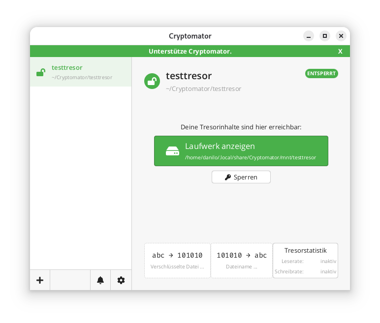
In the locally mounted and decrypted vault, currently only the initial file can be found:
$ ls -l ~/.local/share/Cryptomator/mnt/testtresor
 total 0
 -rw-rw-r-- 1 danilo danilo 471 10. Feb 11:07 WELCOME.rtf
In the actual file system where the vault was created in encrypted form, it looks like this instead:
$ tree ~/Cryptomator/testtresor/
 /home/danilo/Cryptomator/testtresor/
 ├── c
 ├── d
 │   └── KY
 │   └── FEV7TA6N4UV5I3PFT6P7D7DCTNGLDU
 │   ├── dirid.c9r
 │   └── feotyFJDU3AD_3wyOp7Tbd83QUgUGcB46vYT.c9r
 ├── IMPORTANT.rtf
 ├── masterkey.cryptomator
 ├── masterkey.cryptomator.57A62350.bkup
 ├── vault.cryptomator
 └── vault.cryptomator.2BB16E73.bkup
 5 directories, 7 files
The IMPORTANT.rtf file created here only contains a note indicating that it is a Cryptomator vault and a link to the documentation.
Cryptographic Procedures
Cryptomator’s security is based on established, standard-compliant cryptographic procedures:
– Encryption of file contents: AES-256 in SIV-CTR-MAC or GCM mode, depending on the version. This ensures both confidentiality and integrity.
– Encryption of file and folder names: AES-SIV to enable deterministic encryption without opening security vulnerabilities.
– Password derivation: The master key is derived from the user password using **scrypt**, a memory-intensive key derivation algorithm that makes brute-force attacks more difficult.
– Key management: Each vault has a 256-bit encryption and MAC master key. This is encrypted with the Key Encryption Key (KEK) derived from the password and stored in the `masterkey.cryptomator` file.
Further details on the cryptographic architecture are described in the official documentation.
Integration of Third-Party Services
Cryptomator distinguishes between desktop and mobile clients regarding cloud integration.
On desktop systems (Windows, macOS, Linux), integration works via the local synchronization folder of the respective cloud provider. Since Cryptomator only encrypts a folder and does not perform direct network communication, compatibility is very high. Any provider that provides a local folder (e.g., Dropbox, Google Drive, OneDrive, Nextcloud) can be used. Aside from this, an official [CLI client](https://github.com/cryptomator/cli) is also available. However, this appears to be less actively developed than the GUI client; at least the last commit and release are already more than six months old.
On mobile devices (Android, iOS), integration takes place either via native APIs or via the WebDAV protocol. Supported providers such as Dropbox, Google Drive, or OneDrive are offered directly in the app. For other services that support WebDAV (e.g., Nextcloud, ownCloud, MagentaCLOUD, GMX, WEB.DE), a connection can be established manually via the WebDAV interface.
A current list of supported services is available here.
Important Notes on Integration
– WebDAV and Two-Factor Authentication (2FA): For providers with 2FA, an app-specific password is often required, as the main password cannot be used for WebDAV.
– pCloud: WebDAV is disabled when 2FA is activated, which makes use via Cryptomator impossible.
– Multi-Vault Support: Multiple vaults can also be managed in parallel in the client.
External Security Validation of the Project
In 2017, Cryptomator underwent a comprehensive security audit by the recognized security company Cure53. The test covered the project’s core cryptographic libraries, including cryptolib, cryptofs, siv-mode, and cryptomator-objc-cryptor. The audit was predominantly positive: the architecture was rated as robust and the attack surface as very small.
One critical finding concerned unintentional public access to the private GPG signing key, which has since been resolved. Another less critical note referred to the use of AES/ECB as the default mode in an internal class, which, however, was not used in the main encryption path.
The full audit report in PDF format is publicly available.
This is the only publicly available audit of the project that the author could find. However, since audits are generally expensive and time-consuming, the project should be credited for having it conducted and made publicly available.
All other known security issues are also listed on the project’s GitHub page and are visible to everyone.
Conclusion
Cryptomator represents a technically sophisticated, transparent, and cross-platform solution for encrypting data in cloud storage or local data. Through the consistent implementation of the zero-knowledge principle and the use of established cryptographic procedures, it offers high security combined with good user-friendliness.
The separation between encryption and synchronization enables broad compatibility with existing cloud services without them having to change their infrastructure. The open-source nature of the software allows for audits and fosters trust in its security.
Even for less technically savvy users who want to maintain control over their data, Cryptomator is one of the best options available thanks to the GUI client. The specific notes regarding the peculiarities of mobile integration and the fact that both the master key and the password must be strictly protected are, of course, still essential.
Update: Proxday will now take place on October 15, 2026. We have moved the date to avoid a clash with the Dutch Proxmox Day of our friends at Tuxis. All other information remains current – the CfP deadline is extended accordingly to July 31, 2026.
Save the Date: On October 15, 2026, we are bringing the Proxmox world together in Mönchengladbach. With Proxday 2026, we are creating an event that goes far beyond our previous formats. While our Virtualization Gathering and Business Breakfast have already provided valuable impetus, it is now time for the ‘Next Level’. We are dedicating a full day to Proxmox VE and finally giving the community the space it deserves – for deep dives, exchange of experiences, and technical innovations.
Proxday is organized by credativ GmbH and is intended as a meeting point by the community for the community. The focus here is on practical exchange of experience, in-depth technical knowledge, and networking among experts. To ensure the program reflects the full spectrum of the Proxmox world, we invite you to actively contribute to shaping the day.
Call for Papers: Share Your Expertise!
The Call for Papers (CfP) is now officially open. We are looking for exciting presentations, technical deep dives, and practical experience reports. Whether you have built a complex infrastructure, developed automation solutions, or successfully migrated to Proxmox – the community benefits from your knowledge.
Possible topics for your submission:
- Proxmox VE & Storage: Best practices for Ceph, ZFS, and high availability.
- Automation & IaC: Proxmox management with tools like Ansible or Terraform.
- Backup Strategies: Use of Proxmox Backup Server in enterprise environments.
- Networking & Security: SDN implementations and security concepts.
- Migration: Strategies and case studies for switching from other hypervisors.
The submission deadline for the Call for Papers is July 31, 2026.
Event Overview
We have chosen the Hotel Palace St. George in Mönchengladbach as the venue. With its combination of classic architecture and modern amenities, the hotel provides the perfect setting for a focused conference and intensive exchange.
- When: October, 15th 2026
- Where: Mönchengladbach (Hotel Palace St. George)
- What: A day full of expert presentations, networking, and community exchange around Proxmox.
Join us now
Take the opportunity to present your projects to an expert audience or to get early information about the event. All details about the Call for Papers and the venue can be found on the official event website.
We look forward to welcoming the Proxmox community to Mönchengladbach in October 2026!
IMPORTANT NOTE:
We have recently been receiving many inquiries regarding the purchase of the premium version of this software mentioned in the article. We do not offer this version and cannot provide assistance with it. As an open-source service provider, we explicitly only handle the open-source version. For questions regarding the commercially distributed product, please contact the manufacturer at https://languagetool.org/de
LanguageTool: Powerful Language Checking on Your Own Network
LanguageTool is one of the leading open-source solutions for grammatical and stylistic text checking. While most users are likely familiar with the cloud-based version, the on-premise (self-hosted) variant is gaining increasing importance – especially for businesses, educational institutions, and organizations with high data protection and control requirements.
The core of LanguageTool is licensed under the GNU Lesser General Public License (LGPL-2.1). This license permits the free use, modification, and distribution of the software, even in commercial environments, provided that changes to the original code are also published under the LGPL. The license is “weak copyleft,” meaning that applications using LanguageTool as a library do not necessarily have to be open source. License information can be found in the official repository on GitHub in COPYING.txt. Third-party components such as dictionaries may be under different licenses (e.g., GPL).
There is an open-source version as well as an extended premium version with additional features such as improved style, semantics, and format checks. A detailed overview can be found on the website. It is important to note that for self-hosted instances, premium features are only available for commercial use and by individual quote. However, this is communicated with difficulty and primarily in the forum upon request. It also appears that not all premium features are available.
Unfortunately, LanguageTool made changes to the use of browser extensions in 2026: a premium subscription is now required for cloud usage. The self-hosted version remains unaffected – here, the browser extension can still be connected to your own server to enable seamless integration into web applications such as email, CMS, or forms.
Features
LanguageTool has a modular design and combines several technologies. These go far beyond the integrated spell checking of, for example, LibreOffice or Thunderbird. However, a much-desired feature is currently not yet available: support for multiple languages within a single document.
Morphological Analyzer & POS TaggerFirst, the text is broken down into sentences and words. Each word receives at least one Part-of-Speech (POS) tag (e.g., noun, verb, adjective). The analyzer also considers inflectional forms, so
“gegangen” (gone) is correctly identified as a past participle.DisambiguatorMany words have multiple meanings (e.g.,
“Bank” as a bench or a financial institution). The disambiguator uses contextual information to select the correct interpretation. This is done either rule-based or statistically and improves the accuracy of subsequent rule application.Rule Engine (XML & Java)
Error detection is based on a combination of:- XML Rules: Simple patterns like “dass instead of das” or “missing comma before weil.” These are easy to write and maintain.
- Java Rules: Complex, context-dependent rules that are programmatically implemented, e.g., for sentence structure or cross-text repetitions.
N-Gram Model (optional)For improved detection of confusions (e.g., “ihre vs. ihre“), an
n-gram model can be added. This uses statistical data from vast text corpora (e.g., Google Books) and compares the probability of word sequences. The n-gram data is not included in the standard package but can be downloaded locally.- User Dictionaries
spelling_custom.txtCustom technical terms can be added to avoid false positives. This is done either via the API or by editing the
. - Markup Support
WithAnnotatedText, HTML, LaTeX, or XML can be processed without distorting position information. - Java API
For direct integration into Java applications,JLanguageTooloffers a powerful interface
Integration
Integration is versatile: in addition to the browser extension, LanguageTool supports APIs for custom applications, plugins for LibreOffice, Microsoft Word, Thunderbird, and direct connection to development tools. The self-hosted solution thus offers maximum flexibility, security, and scalability – ideal for use in sensitive or regulated environments.
A complete list can be found in the following link. Notably absent is a dedicated plugin for the Outlook client. As far as could be ascertained, the effort was probably not justified by the demand. However, there are only older posts in the forum about this. Nevertheless, LanguageTool in the browser also works without problems with Outlook in the browser. The limitation should therefore only affect the desktop client.
Deployment
On Github, you will find various options for installing a self-hosted service. Especially for local installations, a Docker instance is probably the fastest to deploy.
Several images are linked here; the author chose one as an example.
The maintainer also offers various almost ready-to-use copy-paste solutions to start the service. This includes a Docker Compose template to start the service as an unprivileged user and keep the file system read-only:
To use this, the content must be written into, for example, a docker-compose.yml, the ‘ngrams’ and ‘fasttext’ directories created, and permissions adjusted for, for example, the ‘nobody’ user. All subsequent examples were performed on a Debian 13 system.
$ mkdir ~/Programme/Languagetool
 $ cd ~/Programme/Languagetool
 $ mkdir ngrams fasttext
 $ chown  nobody:nogroup ngrams fasttext
Below is the content of the compose-yaml with support for n-grams in German and English. It is important to note that the n-gram data is quite large and requires several GB of storage.
Currently, it is approximately 3 GB for German and 15 GB for English.
services:
 languagetool:
 image: meyay/languagetool:latest
 container_name: languagetool
 restart: unless-stopped
 user: "65534:65534"
 read_only: true
 tmpfs:
 - /tmp:exec
 cap_drop:
 - ALL
 security_opt:
 - no-new-privileges
 ports:
 - 8081:8081
 environment:
 download_ngrams_for_langs: de, en
 volumes:
 - ./ngrams:/ngrams
 - ./fasttext:/fasttext
The service can then be started with the following command:
$ docker compose up -d
 # Das Herunterladen der n-grams kann etwas dauern.
 $ docker ps
 2af60ed08544   meyay/languagetool:latest   "/sbin/tini -g -e 14…"   4 weeks ago   Up 3 hours (healthy)   0.0.0.0:8081->8081/tcp, :::8081->8081/tcp                             languagetool
The service is now available, and the plugins should be able to access it. There is no authentication or similar. Anyone with access to the URL and port can use it.
Conclusion
LanguageTool on-premise combines data protection-compliant text checking with flexible integration. The LGPL-2.1 license allows free use, while comprehensive interfaces enable seamless integration into office and web applications. With the correct configuration, a local server becomes a fully functional, enterprise-grade solution for linguistic checking.